An important indication of a successful visualization is its ability to reveal an unknown (or overlooked) association between different magnitudes, and to lead the viewers to reflect upon the “causal narrative” behind it; or, as is often the case with tools for exploratory analysis of scientific data, to assist its users in the process of model building and hypothesis testing.
The project challenged me to find a way to visually represent correlations between pairs of variables in a consistent way, irrespective of their type. When two variables are numeric, a scatter plot is typically sufficient in representing their qualitative level of dependency. The two plots below, for example, were generated from data in the 2009-2010 National Health and Nutrition Survey, and compare two variables, arm circumference and standing height, with BMI (Body Mass Index) for adult individuals (18-65 years of age):
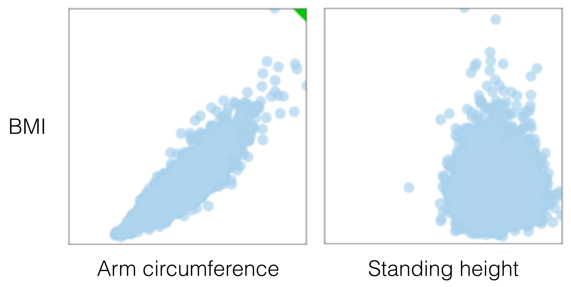
In the first case there is a clear association between arm circumference and BMI, while in the second comparison, standing height is most likely independent from BMI. Visually, a functional relationship between two variables can be identified quite easily, even when there is a large amount of noise in the scatter plot:
If some of the variables are discrete, however, then a scatter plot is not an adequate representation of the information. Below, gender (binary variable) is compared with weight (numeric) and overweight/obese (binary based on the BMI, where its value is “yes” for a BMI greater than or equal to 25, and "no" for the rest of the population).
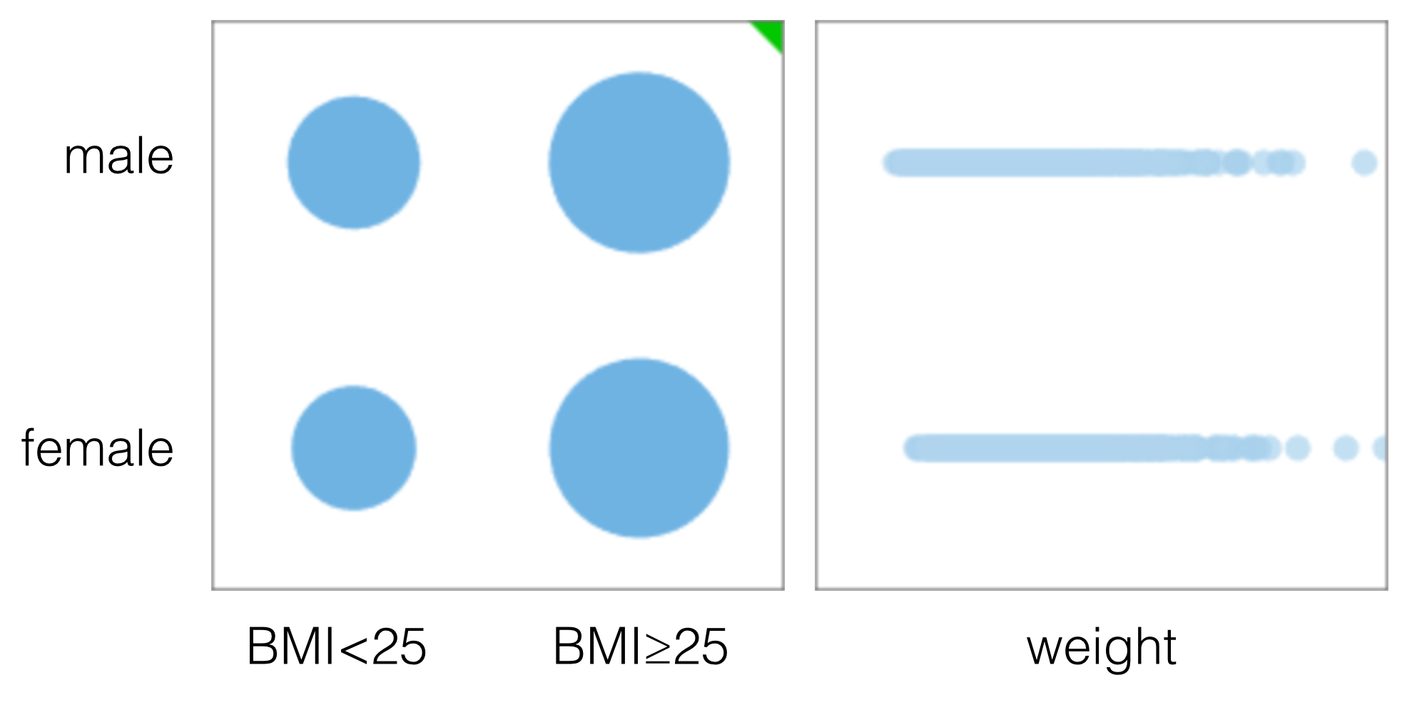
In the first plot, the areas of the circles are scaled to their respective population counts. In both cases, however, it is difficult to visually determine whether the variables are correlated or not. After trying a few alternative representations to solve the limitations of the scatter plot, I found the eikosogram (which I suspect is a special case of the mosaic plot) to be the most effective.
A professor from the University of Waterloo, R.W. Oldford, has written a series of interesting articles about the use of eikosograms to teach basic concepts in probability, as well as to visualize and solve probabilistic problems and paradoxes.
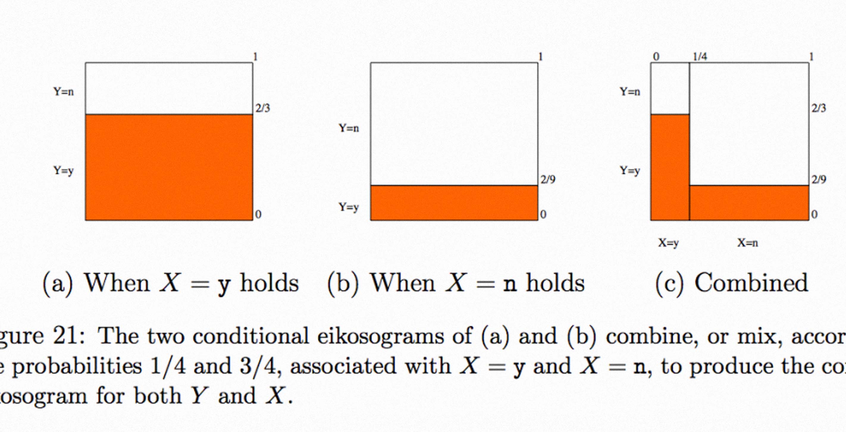
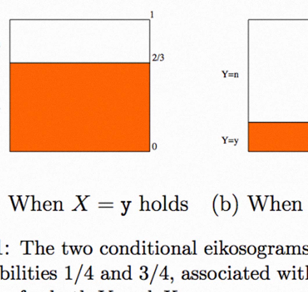
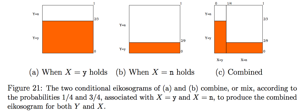
The idea behind the eikosogram is simple, and can be pictured using an image from one of Oldford's papers. If we have two binary variables, say X and Y, and the probabilities of Y=yes when X=yes or X=no are Pr(Y=no)=2/3 and Pr(Y=yes)=2/9 respectively, then the eikosogram of Y given X is pictured on the right:
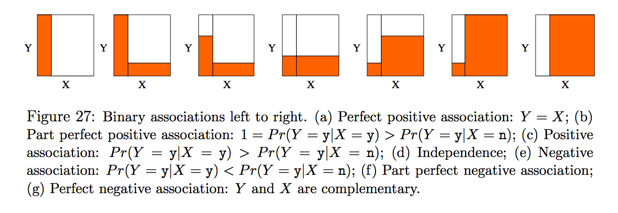
Eikosograms provide a nice visual representation of statistical correlation, because when the two variables are independent, then the value of one, say X, doesn't affect the probability of the second, Y. This visually translates into a horizontal pattern, which easily contrasts with a staircase shape that occurs when the variables are dependent or correlated:
Another motivation for this blog post is to start experimenting with the idea of embedding interactive elements directly inside textual posts, which can complement and expand the written text (if done properly). The p5.js project (a JavaScript interpretation of the Processing language) provided a way to implement a simple eikosogram plot, which you can see below. I have included three datasets that can be explored with the plot. The first two exemplify the association between the incidence of obesity with gender and annual household income among adult individuals in the US. The third dataset contains a list of 1309 passengers from the RMS Titanic, comparing survival rates with cabin class.
You can also load a data file in csv format from your computer by clicking the button below:
The three example datasets are available as downloadable csv files as well: gender-obesity.csv, income-obesity.csv, and titanic.csv
As a final note, it is important to keep in mind that pairwise correlations should be treated with care, not only because of the well-known "correlation does not imply causation" principle, but also due to more subtle effects like the Simpson's paradox. An interactive page from the VUDlab at UC Berkley illustrates this paradox, and represents a good example of combining textual narrative with interactive graphics with the aim of making complex concepts, in this case of statistics, easier to understand.